The main advantage of deep learning is the ability to learn from the data in an end-to-end manner. The core of deep learning is representation, the deep learning models transform the representation of the data at each layer into a condensed representation with reduced dimension. Deep Learning models are often also termed as black-box models as these representations are difficult to interpret, understanding these representations can give us an insight about which feature of the data is more important and will allow us to control the learning process. Recently there has been a lot of interest in representation learning and controlling the learned representations which give an edge over multiple tasks like controlled synthesis, better representations for specific downstream tasks.

Data Representation and Latent Code

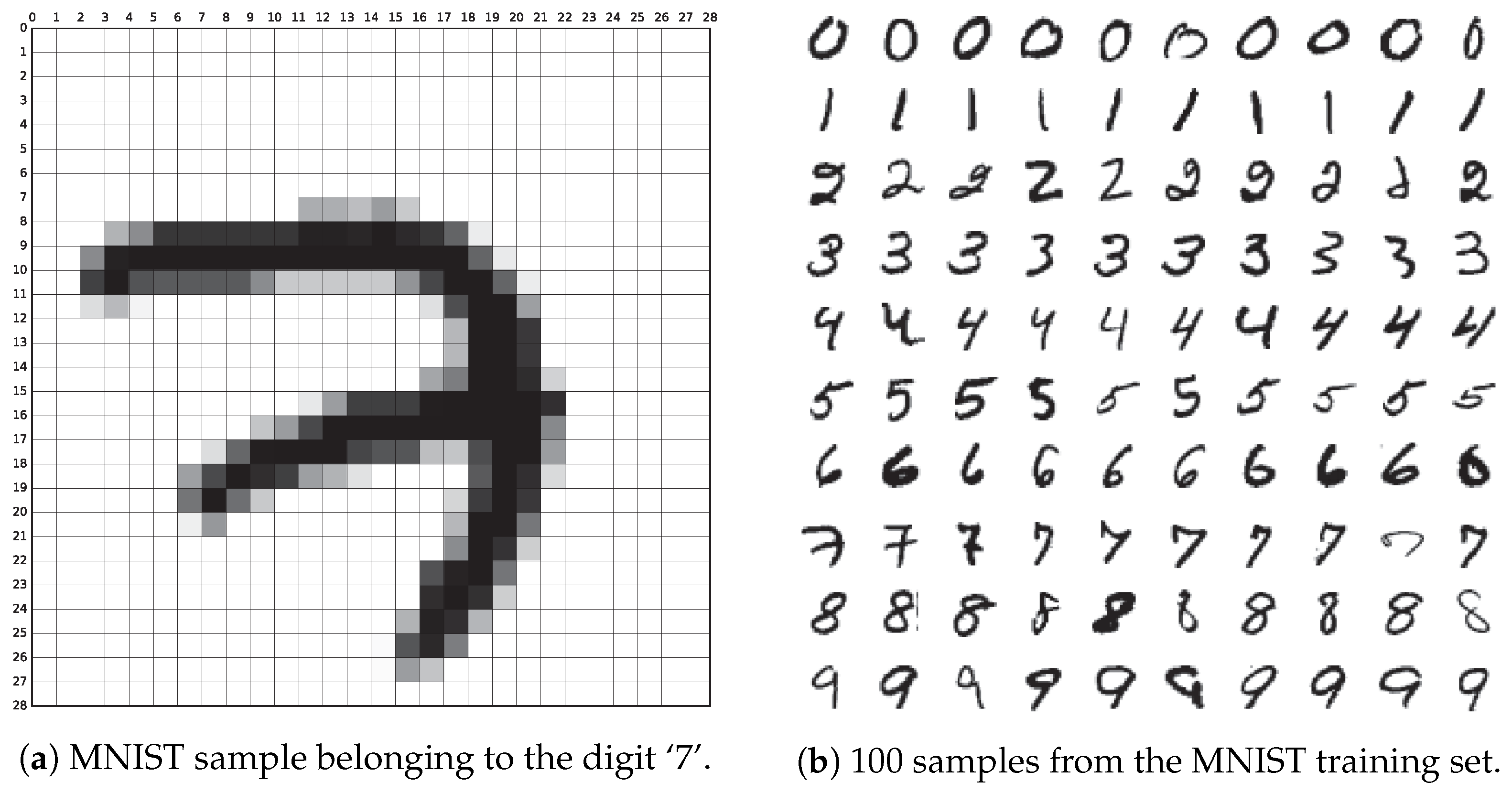
An image \((x)\) from the MNIST dataset has 28x28 = 784 dimensions which is a sparse representation of the image that can be visualized. But all these dimensions are not required to represent the image. The content of the images can be represented in a condensed form using lesser dimensions called latent code. Although the actual image has 784 dimensions \(x \in R^{784}\), one way of representing MNIST image can be with just an integer ie: \(z \in \{0, 1, 2, …, 9\}\). This representation \(z\) reduces the dimension of representing the image \(x\) to 1 which captures the content of which number is present in the image and the variability in the dataset. This is one example of discrete latent code for the MNIST dataset, a continuous latent code will contain more information about the image such as the style of the image, position of the number, size of the number in the image, etc.

Can't See? Something went wrong! — Fig 2: Sample Images of MNIST from [1]

AutoEncoder

Autoencoder[2] models are popularly used to learn such latent code in an unsupervised manner by compressing the image to a fixed dimension code \(z\) and generating the image back using this latent code with an encoder-decoder model.

The encoder \(q_{\phi}(z \mid x)\) of the autoencoder compresses the image to a fixed dimension\((d)\) latent code\((z)\), and the decoder \(p_{\theta}(x \mid z)\) is a conditional image generator. The dimension of z has to be such that, the image can be completely reconstructed by the decoder with the latent code. Choosing the dimension of the latent code is a problem on its own[3].

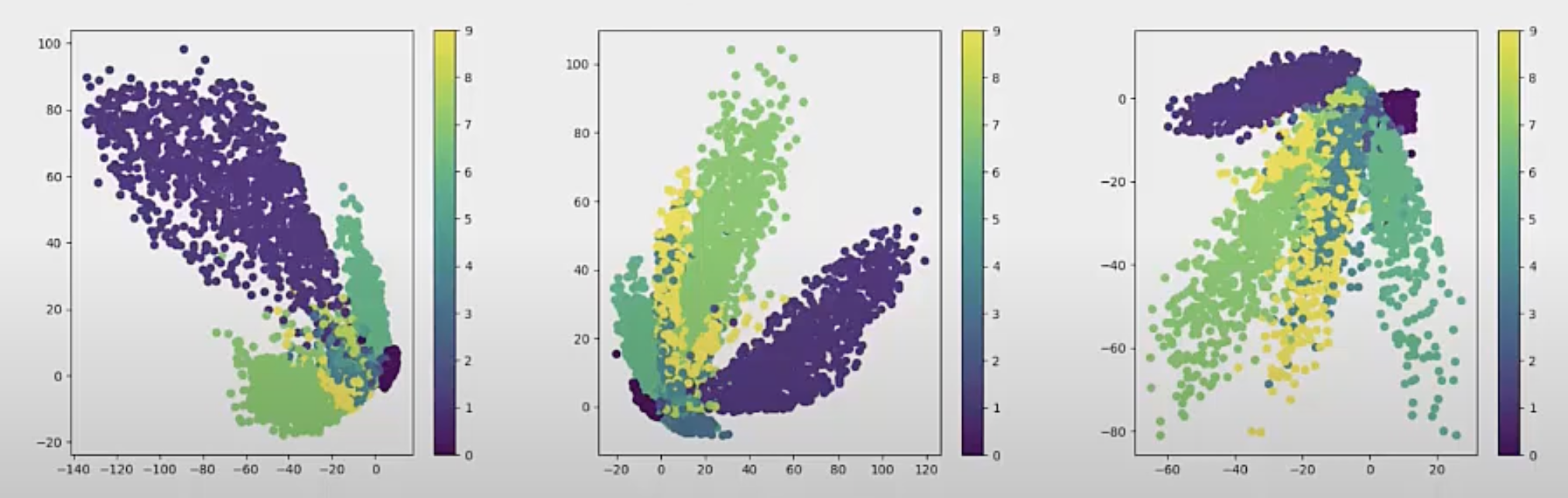
The autoencoder models trained will successfully encode the images into a latent code \(z\), but there is no guarantee that the latent code can be easily inferred, ie: we do not know where in the d-dimensional space the model encoded the image into, and thus difficult to choose a latent code to generate image during inference. So the conclusion is we have no idea how and where the encoder encodes the images, so we do not have control over synthesis during inference. The following figure shows the latent code learned by the AutoEncoder model with different training, as we can observe the latent space keep changing the range and quadrant and thus difficult to infer.

Variational AutoEncoder(VAE)

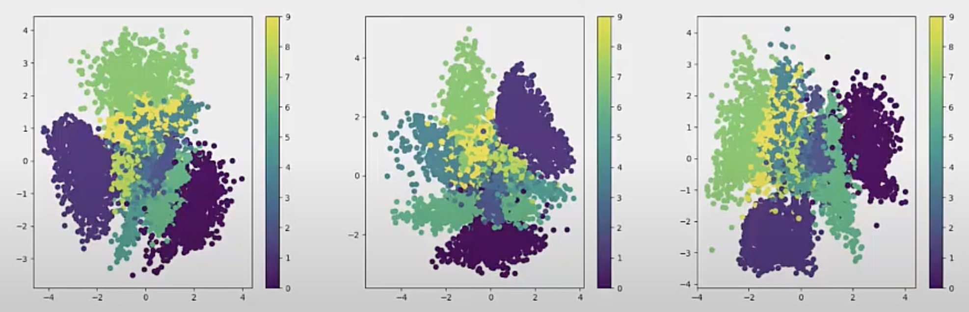
Variational autoencoders(VAE) [6] solve this problem by forcing the latent code (z) to be close to a known prior distribution(Gaussian), this gives us control over the latent space. During inference, the latent space can be sampled from this known distribution for image generation. The following figure shows the latent code learned by VAE with different training, and the latent space across training is centered to the mean 0 across dimensions.

VAE allows us to have control over the latent space and sample from the known prior distribution. But this again does not give us control over the generation of the image. Say if you want to generate an image of the number ‘3’ or ‘7’, you cannot do that(at least not directly). This is where the term “disentanglement” comes into play.

Disentanglement

Feature disentanglement is isolating the source of variation in observation data. There is a lot more factors/feature of an MNIST image other than the number itself, such as the location of the number in the image, size of the image, angle of the number, etc. These factors are independent of each other.

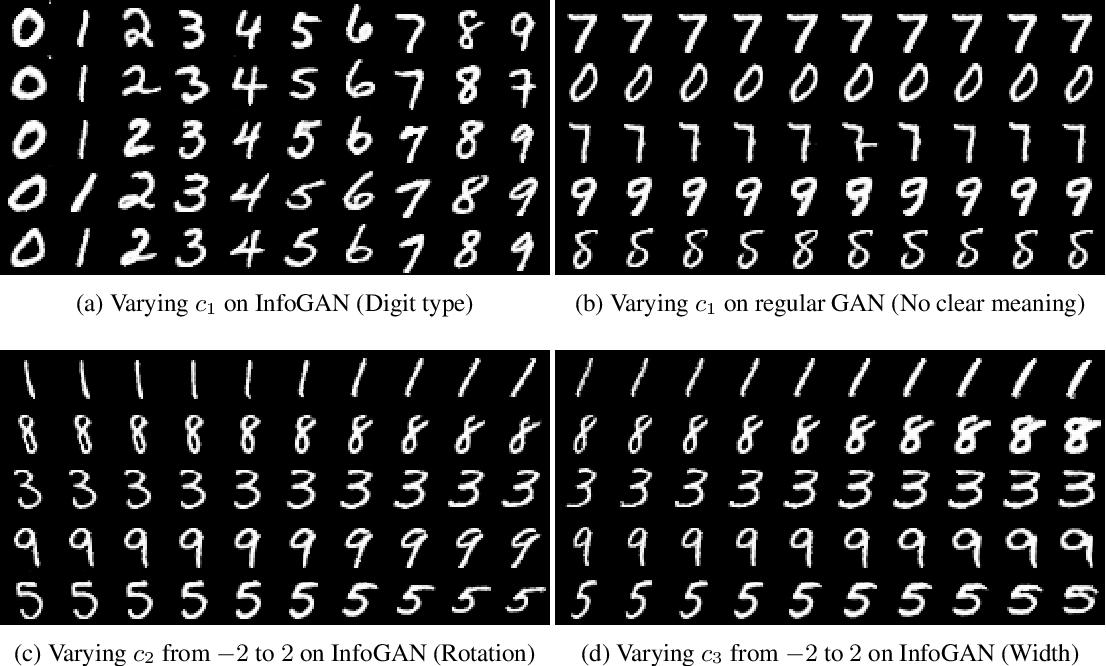
Feature disentanglement involves separating underlying concepts of “Big one in the left”: ie: size(big), number(one), location(left). Our interest here is to see if we can isolate these factors in the latent code so that we can have control over the generation of the images. So we want the encoder to disentangle the representation into different factors and then we generate the image with desired factors say “small seven in the top rotated 30 degrees”.

Beta-VAE

Beta-VAE is a variant of VAE which allows disentanglement of the learned latent code. Beta-VAE adds hyperparameter to the loss function which modulates the learning constraint of VAE.

The first part of the loss function takes care of the reconstruction of the image, it is the second term that learns the latent code of VAE. Different dimensions that span across Gaussians are independent, so by making the prior distribution gaussian, we force the dimensions of the latent code to be independent of each other. So increasing the weight of the second part of the loss, makes the latent code to be disentangled and independent. But this also brings a tradeoff between disentanglement and the reconstruction capability of the VAE. Although Beta-VAE models are good in disentangling the features, the reconstruction ability of this model is not the best.

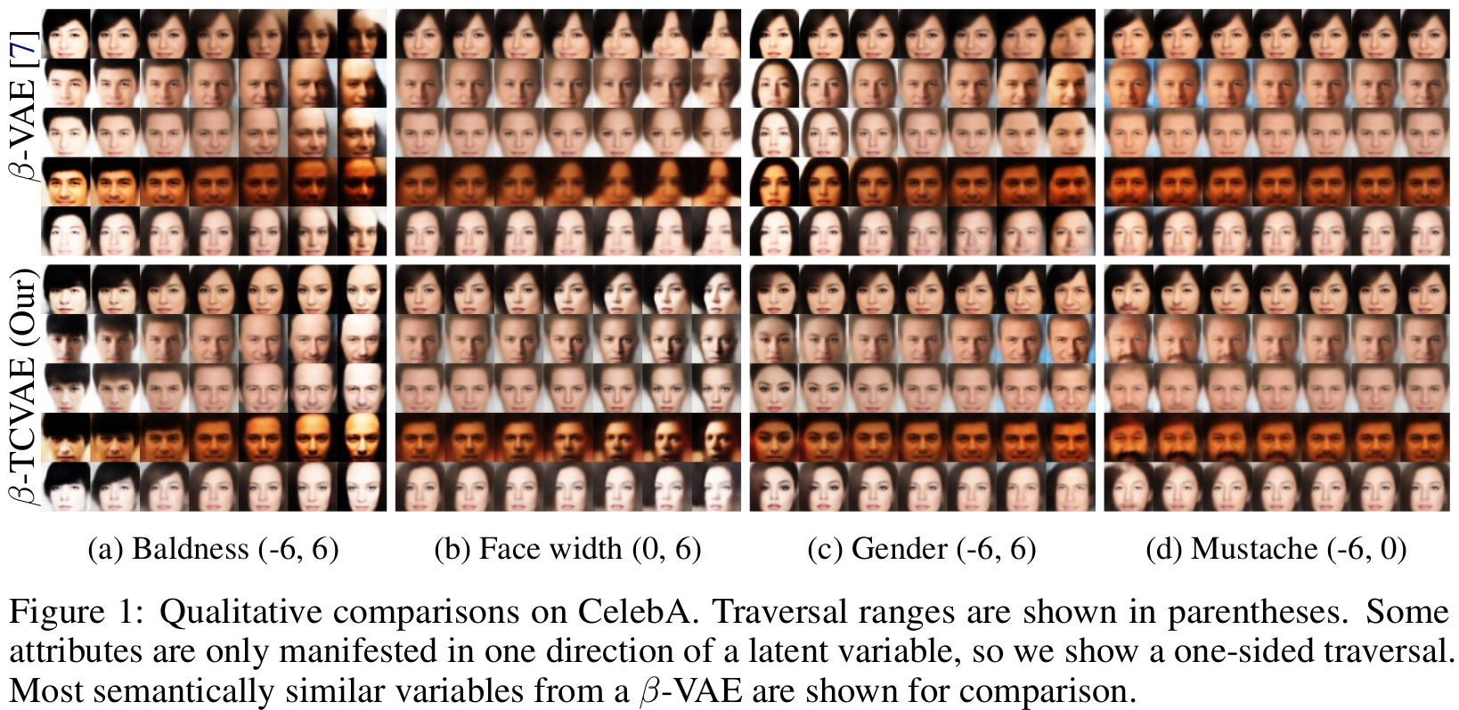
Beta-TCVAE

beta-TCVAE decomposes the KL divergence[10] term of the loss function of VAE into reconstruction loss, Index-code mutual information[8] between data and latent variable, Total Correlation[9] of z, and Dimension wise KL divergence[10] of \(z\)(respectively in the following formula). This helps to break the overall KL Divergence of \(z\) into dimension-wise quantities, which will focus on each dimension of the latent code \(z\). In this formulation, the beta hyperparameter is only on the Total Correlation term which is more important for disentanglement without affecting the reconstruction. So, Beta-TCVAE has better reconstruction ability than Beta-VAE with similar disentanglement property.

\[\mathcal{L}_{\beta-\mathrm{TC}}:=\mathbb{E}_{q(z \mid n) p(n)}[\log p(n \mid z)]-\alpha I_{q}(z ; n)-\beta \operatorname{KL}\left(q(z) \| \prod_{j} q\left(z_{j}\right)\right)-\gamma \sum_{j} \operatorname{KL}\left(q\left(z_{j}\right) \| p\left(z_{j}\right)\right)\]

where \(\alpha = \gamma = 1\) and only \(\beta\) is varies as the hyperparameter.

References :

[1] : A Survey of Handwritten Character Recognition with MNIST and EMNIST (2019)
[2] : Autoencoders (2021)
[3] : Squeezing bottlenecks: Exploring the limits of autoencoder semantic representation capabilities (2016)
[4] : Disentangled Representations - How to do Interpretable Compression with Neural Models (2020)
[5] : InfoGAN: Interpretable Representation Learning by Information Maximizing Generative Adversarial Nets (2016)
[6] : Auto-Encoding Variational Bayes (2013)
[7] : beta-VAE: Learning Basic Visual Concepts with a Constrained Variational Framework (2017)
[8] : Isolating Sources of Disentanglement in Variational Autoencoders