In Part-1, we introduced the concept of normalizing flows. Here, we discuss the different types of normalizing flows. In most blogs that discuss Normalizing Flows, several concepts related to autoregressive flows and residual flows aren’t discussed very clearly. We hope to simplify the explanations of a relatively theoretical topic and make them accessible.
Topics Covered:
- Element-wise Flows
- Linear Flows
- Planar and Radial Flows
- Coupling Flows
- Autoregressive Flows
- Masked Autoregressive Flows
- Inverse Autoregressive Flows
- Residual Flows
- Convolutions and NFs
Element-wise Flows
This is the simplest normalizing flow. In this case, the bijective function \(T\) can be broken into individual components i.e. \(T(x_1, x_2...x_d) = (h_1(x_1), h_2(x_2)...h_d(x_d))\) s.t. every \(h_i\) is a transform from \(R \rightarrow R\). Each dimension has its own bijective function. However, these simple flows don’t capture any dependency between dimensions. Some activation functions like Parametric Leaky RELU (bijective) can be considered element-wise NFs.
Linear Flows
Linear flows are able to capture correlations between dimensions and are of the form : \(T(x) = Ax+b\) , where \(A \in R^{D*D}\) and \(b \in R^D\) where \(D\) is the dimensionality of the input. For the transform T to be invertible, only the matrix A needs to be invertible. When matrix A is a non-diagonal matrix, it captures correlation between different dimensions.
Linear flows are limited in their expressive power. Starting out with a Gaussian \(z \sim N(\mu, \sigma)\), we simply arrive at another Gaussian \(z' = N(A*\mu+b, A^T*\sigma*A)\), similarly for other distributions.
However, they serve as important building blocks for NFs. In terms of computational complexity, computing the determinant and inverse are both of order \(O(D^3)\) where \(D\) is the dimensionality of matrix A. To make the calculation more efficient, there need to be some restrictions on A.
Possible restrictions on A:
- A is a diagonal matrix: this reduces computation time for the calculation of the det. and inverse to \(O(D)\). However, this is equivalent to element-wise bijections.
- A is a triangular matrix: It is more expressive than a diagonal matrix. The computation time for calculation of the determinant is \(O(D)\) and for the inverse is \(O(D^2)\).
- A is an orthogonal matrix: Inverse of an orthogonal matrix is simply its transpose and the determinant is either \(\pm 1\).
There are some other methods that use LU factorisations, QR decomposition which essentially exploit matrix properties to make the computation of inverse and determinant efficient and at the same time allow A to be more expressive.
Planar and Radial Flows
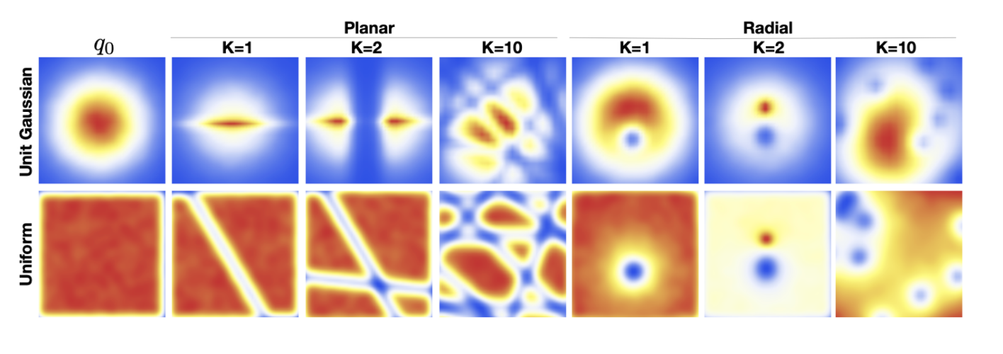
They were first introduced in Rezende and Mohamed [2015], but aren’t widely used in practice and therefore not covered in details here. Planar flows expand/contract the distribution around a certain direction (specified by a plane) and radial flows modify the distribution around specific points. The effect of the flows can be seen below. The left half shows the effect of planar NFs on an initial distribution of a Gaussian and uniform distribution, and the right half shows the effect of a radial flow.
Coupling Flows
Coupling flows are highly expressive and widely used flow architectures. They can either have linear or non-linear invertible transformations.
Coupling flows are defined by two sets of mappings, an identity map and a coupling function \(h\). Consider a disjoint partition of the input \(x \in \mathbb{R}\) into two subspaces: \((x^A, x^B)\) \(\in\) \(\mathbb{R}^d \times \mathbb{R}^{D-d}\). A bijective differentiable coupling function is defined as, \(h(\cdot ;\theta)\) : \(\mathbb{R}^d \rightarrow \mathbb{R}^{D}\) that is parameterized by \(\theta\). The equations for both the mappings are shown below.
\(y^A\) = \(h(x^A, \theta(x^B))\)
\(y^{B}\) = \(x^B\)
The bijection \(h\) is called a coupling function, and the resulting function \(g\) that consists of both the mappings is called a coupling flow. Coupling flow is invertible if and only if \(h\) is invertible and has an inverse.
Let’s consider an example :
Let us consider an input with 4 dimensions \((x1,x2,x3,x4)\). Let \(x^A = (x1,x2)\) and \(x^B = (x3,x4)\). Let \(\theta(x^B) = x3+x4\) and let the coupling function \(h(x^A, \theta(x^B)) = \theta(x^B) * x^A\).
Given this example, the coupling function \(h\) is invertible but only if \(\theta\) isn’t zero. Therefore, the invertibility requirement of \(h\) introduces a limitation on \(\theta\) as well. In this case, it can’t be defined as a simple additive function. The restriction for non-zero values needs to be taken into account.
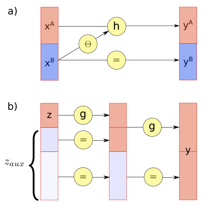
The figure above shows two examples of coupling flow architectures. In figure (a), \(x^{A}\) and \(x^{B}\) are the two input subspaces. The coupling function \(h\) is applied to \(x^{A}\) directly while it is parameterized on \(x^{B}\). In figure (b), there are two subsequent flows, where the size of input subspace on which the coupling function \(h\) is applied, gradually increases with each flow.
There are various types of coupling functions. We discuss some of these briefly,
- Additive coupling
- This is one of the simplest form of coupling functions defined by, \(h(x;\theta) =\) \(x + \theta\), where \(\theta\) is a constant \(\in \mathbb{R}\)
- Affine coupling
- \(h(x;\theta) =\) \(\theta_1x + \theta_2\), \(\theta_1 \neq 0\), \(\theta_2 \in \mathbb{R}\) Both additive and affine coupling were introduced in NICE.
- Neural auto-regressive flows
- This was first introduced by Huang et al [2018]. The coupling function \(h(\cdot;\theta)\) is modelled as a neural network. Every neural network can be considered as a parameterized function, the parameters being the weights. In this case, the weights of the neural network are defined by \(\theta\). To ascertain that the neural network follows bijectivity, the following proposition is applied :
- If \(NN(\cdot)\) : \(\mathbb{R} \rightarrow \mathbb{R}\) is a multilayer perceptron, such that all weights are positive and all activation functions are strictly monotone, then \(NN({\cdot})\) is a strictly monotone function. So, since the neural network is monotone, it is also invertible and hence a normalizing flow.
- This was first introduced by Huang et al [2018]. The coupling function \(h(\cdot;\theta)\) is modelled as a neural network. Every neural network can be considered as a parameterized function, the parameters being the weights. In this case, the weights of the neural network are defined by \(\theta\). To ascertain that the neural network follows bijectivity, the following proposition is applied :
More types of coupling flows can be found in this paper.
Autoregressive Flows
An autoregressive flow is a type of normalizing flow where the transformations use autoregressive functions. The term autoregressive originates from time-series models where the predictions at the current time-step are dependent on the observations from the previous time-steps.
The probability distribution of an autoregressive model is given by, the equation below where the output at time-step \(i\) is conditioned on all the previous outputs.
\[p(x) = \prod_{i=1..D} p(x_i | x_{1:i-1})\]An autoregressive function can be represented as a coupling flow:
Let the coupling function \(h(\cdot ;\theta)\) : \(\mathbb{R} \rightarrow \mathbb{R}\) be a bijection parameterized by \(\theta\), and let \(x_{1:t}\) be the set of inputs Then, an autoregressive model is a function \(g : \mathbb{R}^D \rightarrow \mathbb{R}^D\), in which every entry of the output \(y = g(x)\) is conditioned on the previous entries of the input:
\[y_t = h(x_t ; \theta_t(x_{1:t-1})\]The functions \(\theta_t(\cdot)\) are called conditioners. \(\theta_1\) is a constant whereas \(\theta_2\), \(\theta_3\) … , \(\theta_t\) are arbitrary functions mapping \(\mathbb{R}_{t-1}\) to the set of all parameters. The conditioners need to be arbitrarily complex for effective transformations and hence, are usually modelled as neural networks.
Since each output depends only on the previous inputs, the Jacobian matrix of an autoregressive transformation \(g\) is triangular (refer to Part 1 for explanation). The determinant of a triangular matrix is simply a product of its diagonal entries.
\[\det{(Dg)} = \prod_{t=1..k} |\frac{\partial y_t}{\partial x_t}|\]Masked Autoregressive Flows (MAFs)
The time taken to train autoregressive flow models is very high because of the need to sequentially generate outputs. Using MAFs one can parallelize the training process.
MAFs were inspired by the observation that on stacking several autoregressive models, where each model had unimodal conditionals, the normalizing flow can learn multi-modal conditionals (MAF [2018]). The architecture consists of stacked MADEs with Gaussian conditionals which are explained below.
What are MADEs?
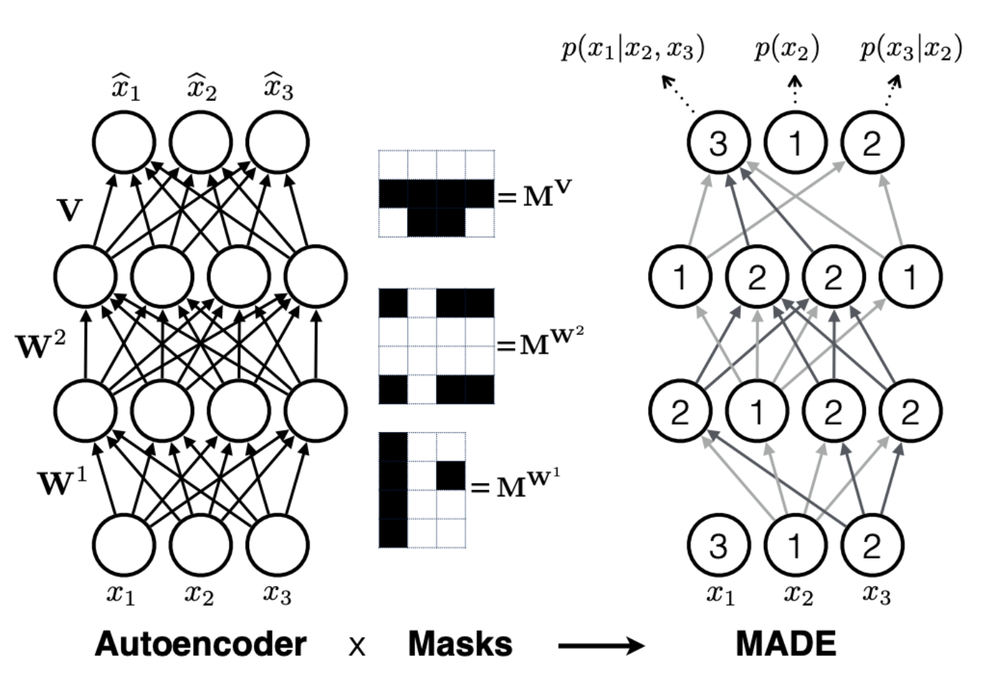
MADE stands for Masked Auto-Encoder for Distribution Estimation (MADE [2015]) are essentially auto-encoders with some modifications like masks. In a MADE, the autoregressive property is enforced by multiplying the weight matrices of the hidden layers of the auto-encoder with a binary mask. These masks ensure that the training of the sequential auto-regressive model can be done in parallel.
The masking is done such that forward passes with mask are equivalent to conditioning the output only on the earlier sequences of input. This is shown in the below image. On the left, a typical auto-encoder with 2 hidden layers is shown. If one wants to represent the output as an autoregressive sequence specified by the equation below, then masks are multiplied to the weights of the auto-encoder.
\[p(x) = p(x_2) * p(x_3 | x_2) * p(x_1 | x_2, x_3)\]The order of the inputs are \(x_2, x_3, x_1\) The image on the right shows the network weights after masking. For example \(p(x_2)\) doesn’t depend on any of the other inputs since it is the first in the sequence. \(p(x_3)\) is dependent on only the nodes that depend on \(x_2\) and similarly for \(p(x_1)\) The general form for masking is discussed in the MADE paper. The MADE architecture parallelizes the sequential autoregressive computation.
Density Estimation and Sampling
There are two important concepts when studying flow architectures : density estimation and sampling. Both these passes have different computation complexity and for auto-regressive models, the computation time of one is inversely related to the other.
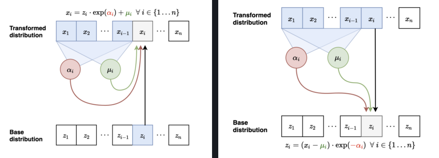
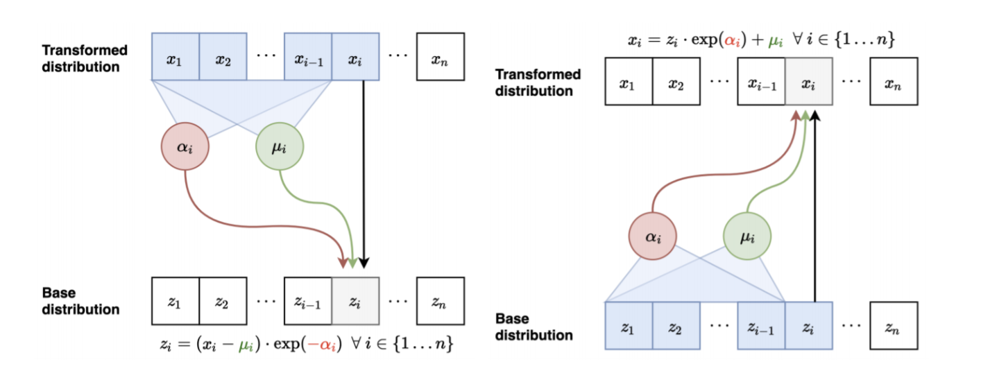
The diagrams above demonstrate a forward pass and an inverse pass in a MAF. The output \(x_i's\) depends upon the input \(z_{i}\) and the scalars \(\alpha_{i}\), \(\mu_{i}\) which are computed using \(x_{1:t-1}\). It is these scalars that define the density parameters of the distribution. This is also called a scale and shift transform. The reason why it is designed this way is that inverting \(f(x)\) does not require us to invert the scalar functions \(\alpha_{i}\) and \(\mu_{i}\).
\(f^{-1}(x_{i}) = z_{i} = \frac{x_{i} - \mu_{i}}{exp(\alpha_{i})}\).
MAFs can compute the density \(p(x)\) very efficiently. During the training process, all the \(x_i's\) are known. One can therefore parallelize this step using masks. Sampling on the other hand (predicting \(x_{D}\)) is slower as it requires it requires performing \(D\) sequential passes (where \(D\) is the dimensionality of \(x\)) to calculate the previous samples (\(x_{1}, x_{2} ... x_{D-1}\)) before computing \(x_{D}\).
Inverse Autoregressive Flows (IAFs)
Since MAFs are better at training by exploiting parallel computation but slower during sampling, we modify the functions to get another flow architecture that is faster at sampling. This gives us Inverse Autoregressive flows (IAFs).
The figures above show a comparison between the inverse pass of a MAF and the forward pass in an IAF. The only difference between both the architectures is that for IAF’s the autoregression is based on the latent variables and not the predicted distribution. The scale(\(\alpha_{i}\)) and shift(\(\mu_{i}\)) quantities are computed using previous data points from the base distribution instead of the transformed distribution.
IAF can generate samples efficiently with one pass through the model since all the \(z_i's\) are known. However, the training process is slow, since estimating the \(z_i\) requires i sequential passes to calculate all the required input variables \(z_{1}\), \(z_{2}\), .. \(z_{i-1}\).
Aside : According to our understanding, during training, both the weights of the network parameters(\(\alpha, \mu\)) and \(z_i's\) are estimated i.e. the ith latent variable is itself treated as a parameter that is to be learned.
One should use IAFs if fast sampling is needed, and MAFs if fast density estimation is desirable.
Parallel WaveNet [2017] which was once the state-of-art model for speech synthesis made use of a MAF and an IAF. A fully trained “teacher” network that used MAF architecture was used to train a smaller and parallel “student” network that used IAF architecture. Since the teacher used MAF architecture it could be trained fast. Once the student network, an IAF model, was trained, it could then generate all the audio samples in parallel without depending on the previously generated audio samples and with no loss in audio quality.
Residual Flows
During training, deep networks find it difficult to reach a convergence point due to the vanishing/exploding gradient. In such cases, adding more layers to the network only results in a higher training error. Residual Networks or ResNets were introduced to solve this problem. ResNets consist of skip-connection blocks.
A residual block is shown below. The output of the residual block is represented by the equation below, where \(F(x)\) represented the pass through the neural layers.
\[M(x) = F(x) + x\]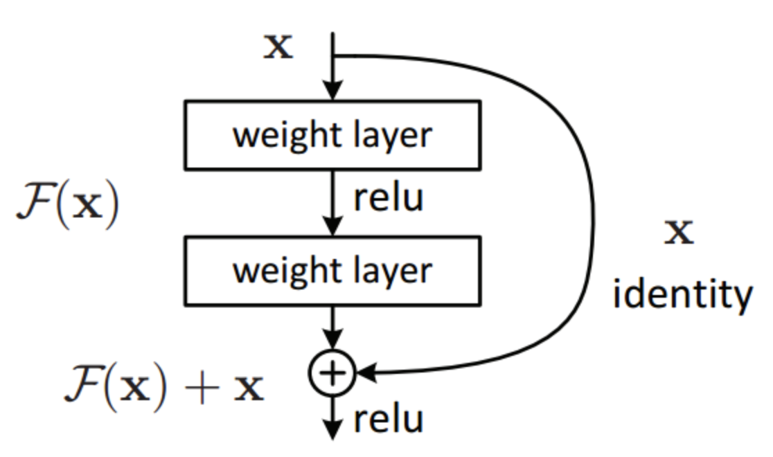
How does this help? Skip connections in a deep neural network allow the back-propagation signal to reach the initial layers of the neural network thereby solving the vanishing gradient problem. Instead of treating the number of layers as an important hyper-parameter to tune, by adding skip connections to our network, we are allowing the network to skip training for the layers that are not useful and do not add value to overall accuracy. In a way, skip connections make our neural networks dynamic, so that they may optimally tune the number of layers during training.
Residual flows in their general form aren’t invertible and can only be used in flow architectures after applying some constraints(first introduced in Chen et al. [2019]). This is discussed next.
A Lipschitz condition is necessary to enforce invertibility in residual flows.
Lipchitz condition : A real valued function : \(f : \mathbb{R} \rightarrow \mathbb{R}\), is Lipchitz continuous if there exists a positive real constant \(K\) such that, for all real \(x_1\) and \(x_2\), \(|f(x_1) - f(x_2)| \leq K| x_1 - x_2 |\)
If \(K = 1\) the function is called a short map, and if \(0 \leq K < 1\) the function is called a contraction.
Invertible Residual Flows: Given a residual flow of the form, \(F(x)=x+g(x)\), if the mapping \(g(x)\) has a lipschitz constant \(K\), \(0 \leq K < 1\) then the residual flow is invertible. We discuss a short proof of this next.
For the residual flow to be invertible, proving that \(F(x)\) is monotonically increasing is sufficient i.e. we need to prove \(F(x+\delta) - F(x) >= 0\)
\[F(x+\delta) - F(x) = x+\delta + g(x+\delta) - (x - g(x)) = \delta + g(x+\delta) - g(x)\]From the Lipschitz condition for \(g\), we have \(|g(x+\delta) - g(x)| \le |\delta|\), since \(0 \leq K < 1\). Therefore, \(F(x+\delta) - F(x)\) is always >= 0 and hence monotonically increasing.
The addition of invertible residual blocks greatly enhances the class of neural network flow models and also ensures we can train deeper models without the fear of vanishing gradient.
Convolutions and NFs
Convolutions are one of the most common operations used in the design of DNNs, however, the computation of their inverse and determinant is non-obvious. Since they aren’t invertible they can’t be used in the family of NF flows. However, recently [Hoogeboom et al. 2019] defined invertible \(d*d\) convolutions and designed an architecture using stacked masked autoregressive convolutions. This is explained next.
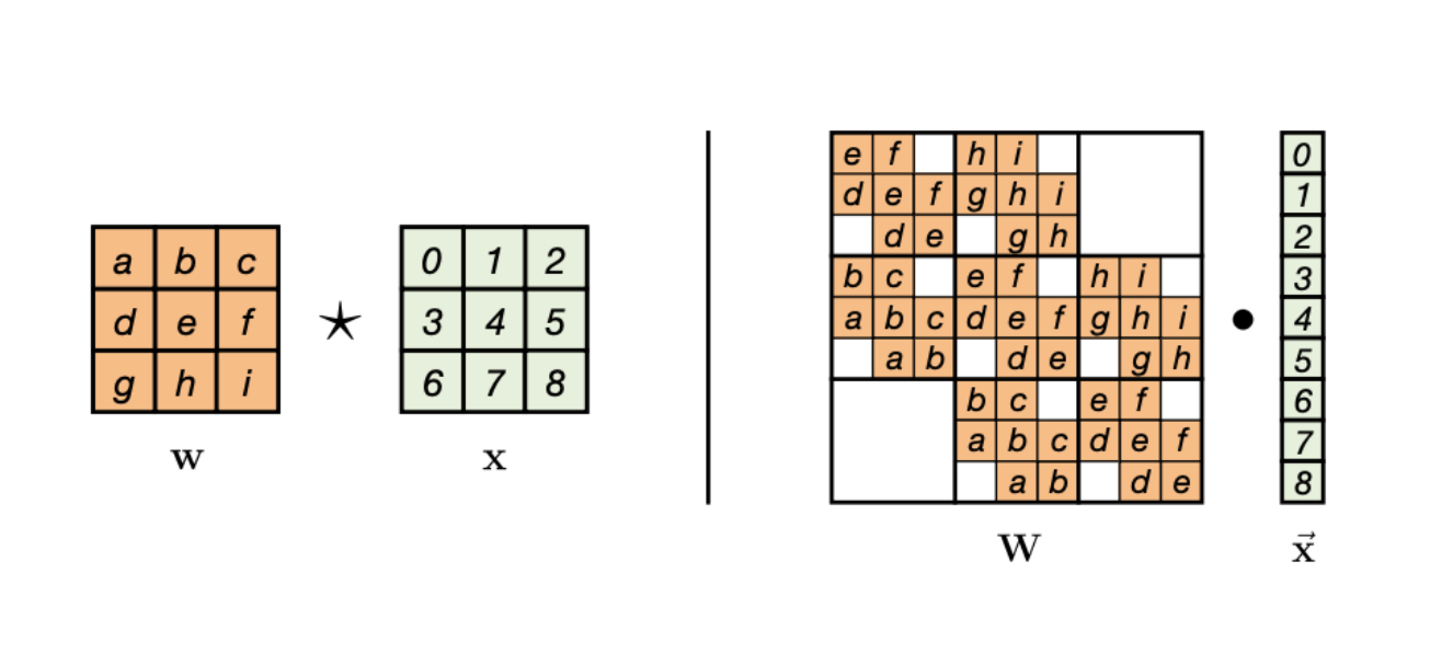
In the figure below, on the right, the input x is shown along with the kernel matrix w. The convolution operation between these two can be represented as a matrix multiplication of the form \(A*x\) shown on the right. The matrix A is non-invertible here, however, if we consider \(f = g = h = i = 0\), then, we get a triangular matrix that can represent a normalizing flow.
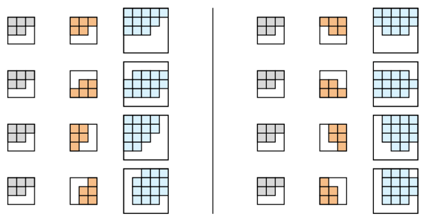
One of the issues of using a filter where \(f = g = h = i = 0\) is that the receptive field is narrow. However, one can rotate the filter and combine two filters to get different receptive fields as shown on the left in the image below. These can then which can be stacked to capture more expressive combinations as shown on the right. These are called “expressive convolutions” in the paper. The grey and orange filters are rotations of the same filter that result in a triangular matrix. They can be stacked to get different receptive fields shown in blue. These blue receptive fields can be stacked further to arrive at more expressive transforms that have the desired receptive field.
This concludes our discussion of normalizing flow architectures. Incase of any doubts/questions please reach out to us at kriti@skit.ai or swaraj@skit.ai.